Small Angle X-Ray Data –
Size Distribution in Alumina Powder
In
this tutorial you will determine the size distribution of particles in an
alumina polishing powder using data from a constant wavelength synchrotron X-ray
USAXS instrument. You will use both Maximum Entropy (MaxEnt)
and Total Non-Negative Least Squares (TNNLS) methods assuming spherical
particles. The data were collected from powders spread onto sticky tape and covered with
another layer of the same tape. The data were corrected for background from
data collected from two layers of sticky tape. However, the sample thickness is
not accurately known so the data are not calibrated on an absolute scale.
If you have not done so already, start GSAS-II.
Step 1: read in the data file
1. Use the Import/Small Angle Data/from q (A-1) step X-ray QIE data file menu item to read the data file into GSAS-II. This read option is set to read three column small angle scattering data (SASD) as Q in Å-1, intensity and estimated standard deviation in intensity; there may be a header with metadata information in the front of this file. Change the file directory to SAsize/data to find the file; you will have to select the ‘any file (*.*)’ filter to see it.
2. Select the alumina data.dat data file in the first dialog and press Open. There will be a Dialog box asking Is this the file you want? Press Yes button to proceed.
At this point the GSAS-II data tree window will have several entries and the plot window will show the SASD pattern as a log-log plot of intensity vs. Q

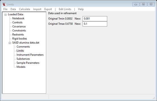
Step 2: Set Limits
For this step we will reposition the limits to enclose only that part of the SASD pattern suitable for size distribution analysis. Typically this covers 10-3 < Q < 10-1; below this range scattering is from very large objects not readily described by the size distribution analysis and above the scattering is mostly background. Select Limits under SASD alumina data.dat from the GSAS-II tree. Then set changed to 0.001 for Tmin and 0.1 for Tmax. You can also set the limits using the cursor on the plot by either picking a point on the curve with the left or right mouse button or by dragging the green and red vertical lines to the desired positions. The limits window should look like
Step 3 Select the scattering substances for your sample
Two scattering substances need to be defined for your sample to give the anticipated scattering contrast; in this case one is alumina and the other is “vacuum” (really air). Parameters for a number of substances are defined in the file Substances.py. You can add your own substances to this or better put them in UserSubstances.py; this is read after Substances.py when you load substances for your selection. Select Substances under SASD alumina data.dat from the GSAS-II tree. Then do Edit substance/Load substance from the menu; a popup window will appear with possible selections

Select Alumina and press OK; the relevant data for alumina (and vacuum) are displayed next

If desired you can load/add as many substances as you want into this list; you can also delete any of them (except vacuum & unit scatter). The composition, volume occupied by the atoms in the composition and the density are given for each substance. These can each be edited; the other values will change accordingly. If your substance isn’t in the list, you can Edit Substance/Add substance to create a new one (you will be asked for a name and the set of elements in two successive popup windows). From this information the scattering density and that as affected by resonant scattering for the listed wavelength is displayed (the wavelength can be changed in the Instrument Parameters GSAS-II tree item if needed). The real density value is used for contrast calculations.
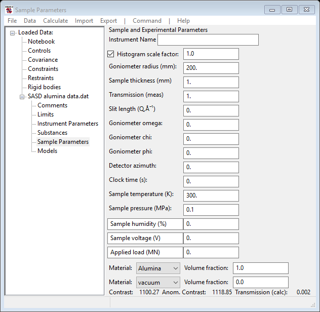
Step 4: Set Sample parameters
Two of the substances you have loaded into GSAS-II next need to be selected for this size distribution analysis; Select Sample Parameters under SASD alumina data.dat from the GSAS-II tree. Near the bottom of the window will be two rows marked “Material”; select Alumina from one of the pull downs (leave the other as vacuum). The window will show at the bottom the computed contrast between alumina and vacuum without and with consideration of resonant scattering effects; the latter is used in subsequent calculations.
For experiments for which you know the transmission and the sample thickness, you can manipulate the volume fractions to make the calculated transmission match the observed one. Additionally, if you have absolute scaling information, you can rescale the data by adjusting the histogram scale factor; multiple data sets can be scaled together via the Command/Set scale menu item.
Step 5 Size distribution via Maximum Entropy
You are now ready to attempt a size distribution analysis using the maximum entropy method. Select Models under SASD alumina data.dat from the GSAS-II tree; the window will display

Many selections are made by default for this analysis; however it is important that an appropriate value is selected for the background. From the high Q end of the data plot
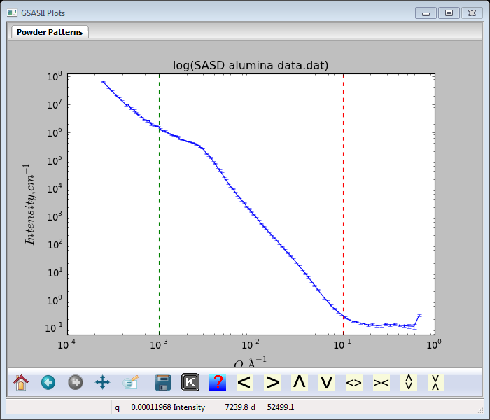
It is clear that the intensity levels off at an apparent background level of ~0.12; enter that into the appropriate place in the data window next to Background. The plot will be redrawn showing a horizontal red line for the background. All the other parameters seem reasonable for a 1st attempt at a MaxEnt solution. Do Models/Fit; the console window will show that the calculation did not converge and the Size Distribution plot has a “choppy” appearance.
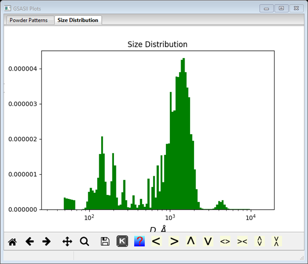
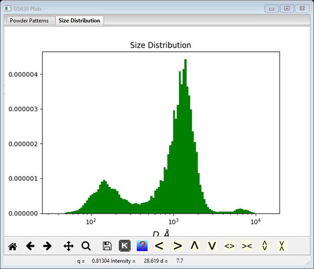
This is not a satisfactory result, but the suggestion given in the console window is worth trying. Change the Error multiplier to 5 (notice the increased error bars on the data plot) and repeat Model/Fit. Convergence is now achieved in <10 cycles (see console window for details) and a much smoother size distribution results

This is a good result: clearly the alumina polishing powder has a bimodal distribution with diameters centered about ~1600Å and ~160Å (not 500Å and 1µm as advertised by the manufacturer!).
You may wish to explore the effect of some of the other parameters in the data window. Most are obvious but Log floor factor needs a bit of explanation. This is the log of the minimum size distribution (scaled by the histogram scale factor and the contrast). This size distribution minimum needs to be set within 1-2 orders of magnitude of the optimal value and can differ from the default of 10-3; it is worth changing if convergence is poor despite trying different error multipliers. Try changing it to see what effect it has on the result. With the original settings the data fit looks like
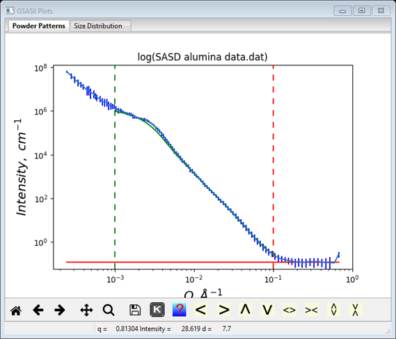
The green curve is the result calculated from the size distribution. Notice that it is not perfect, there is appreciable misfit around Q=0.003Å-1. This may be due to the assumption that the particles are spheres; they could be some other shape (I could get a better fit by setting the Spheroid aspect ratio to 2.0), however this tool is not really the appropriate one to make this determination.
Step 6 Size Distribution via Total Non-Negative Least Squares (TNNLS)
An alternative method for determining size distributions is the TNNLS or Interior-Point Gradient (IPG) method. As the name implies this is a gradient refinement method for the special case of all positive data and parameter values. To try it on this alumina data, select IPG from the Fitting method pull down. The data window will change to give
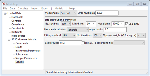
Reset the Error multiplier back to 1.0 and then do Models/Fit to run the IPG fitting. The IPG algorithm did not converge in 100 cycles and resulting size distribution is a little choppy but has roughly the same bimodal distribution found by MaxEnt.

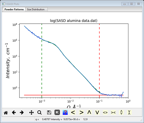
This can be considerably improved by setting the Error
multiplier to 2.0; the IPG fit converges in <20 cycles and gives a smoother size
distribution.
The bimodal distribution is again quite clear with ~1400Å and ~150Å diameter particles. This method appears to give a better fit to the data than the MaxEnt method particularly in the Q~0.003Å-1 region’
You may wish to explore the other parameters for the IPG fitting. If Q power weight is set to 0-4, that changes the data weighting to Qp. This can change the convergence of the IPG method and yield improved results if one is unsuccessful with the default settings. I got a nice fit with a Q power weight of 3 and Error multiplier of 2.0.
You should save this GSAS-II project as it will be used in the tutorial for fitting small angle scattering data; I used alumina.gpx.